

Auto-Correlation & Stationarity
Auto-Correlation & Stationarity
The effect of 'Fractional Differencing' on stationarity and auto-correlation.


This is a follow-up to my previous article, “What are Regimes?”, which describes variational inference based clustering for time series data. In this post, I will demonstrate clustering with that method on fractionally differentiated price data and how this effects the stationarity, auto-correlation and clustering properties of the data.
Stationarity, Auto-Correlation, & Differencing
Stationarity is the property of a time series that its statistical properties remain constant over time. If a time series has a mean, variance, or any other statistical parameter that is inconsistent through time, it is not stationary over that parameter. Typically as being measured by some type of moving window that measures important shifts in time.
Weak and strong forms of stationarity exist depending on which statistical properties are invariant and to what degree. Typically, we are at least very interested in the mean or possibly the variance.
Auto-correlation refers to the correlation of a time series with its lagged self. If large perturbations in a time series tend to be followed by more large perturbations for a period of time, then that might cause the time series to drift away from its previous statistical parameters, introducing non-stationarity through the auto-correlation or autoregressive process.
Differencing is used to make a time series stationary again despite such perturbations such as with Python's np.diff function. By taking the difference between consecutive values, np.diff removes the unit root in the data and can make a time series stationary (given that the order of differencing matches that unit root).
Making a series stationary will also reduce auto-correlation by removing the dependence between values in the time series, if it was produced by an autoregressive term.
Unit Root Stochastic Process
A unit root is a feature of a time series process such as an AR(1) process where the autoregressive lag is produced by a characteristic root value. It is a characteristic of non-stationary time series, where the mean of the series is not constant over time.
Mathematically, a time series with a unit root can be expressed most simply as,
There is an error term which is noise, and the term producing the unit root with a characteristic root value, which we will consider as 1 such that differencing one time is enough to remove the unit root. Here we consider the simple base case.
Any perturbation (any non-zero value for the noise term) shifts the time series off it’s previous trend or mean and it does not revert. This is the definition of a basic unit root stochastic process, which is much like the random walk of a stock price. Although stock prices do exhibit short term trends, in the long run their trends are constantly shifting in unpredictable ways, and they do not mean revert to a single well-defined trend.
The next periods stock price is always just a function of the current period price plus some noise: the completely unpredictable stochastic component of the price movement. This noise still has variance sigma squared and it is heteroskedastic. After 1st-order differencing of the process, we are left with only the Gaussian noise that is stationary by the mean but may still be non-stationary by the variance.
Fractional differentiation, as described next, using a value less than 1 will ultimately not completely remove the unit root — it will leave some intact. The ADF test (Augmented-Dickey Fuller) is used to test for a unit root in time series.
Fractional Differentiation
In Machine learning tasks, we often need the data to be stationary to learn meaningful generalizations of it. But at the same time, we know that auto-correlation by its very construction gives the data some predictability and memory. Fractional differentiation provides a controlled method of balancing between these two priorities: preserving some auto-correlation and memory while also making the series stationary.
First the series is fractionally differenced as described by Marcos Lopez de Prado in Advances in Financial Machine Learning. As opposed to the traditional derivative approach, taking the rate of change between time points, imagine that we take a fractional rate of change.
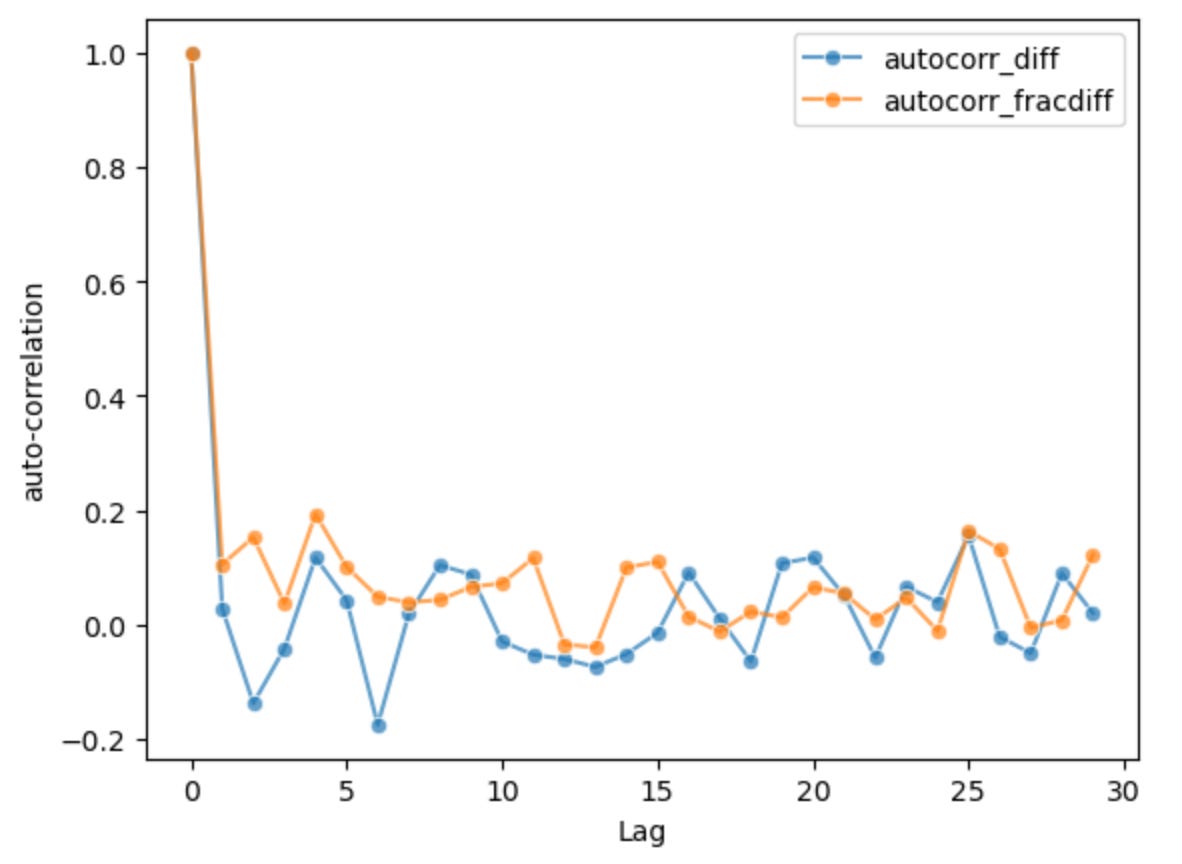
In this notebook I work with a small sample of intraday price data (one full day’s minute-level data). A fractional order value of 0.9 is used. The auto-correlation plots show that the memory of the series decays more slowly after this transformation, versus the standard 1st-order differenced data. What we’ve done is attenuated the effect of the unit root.
Notebook: https://github.com/regimelab/notebooks/blob/main/fractional_differentiation.ipynb
References & Further Reading
Advances in Financial Machine Learning
Marcos Lopez de Prado
Long Memory and Regime Switching
Francis X. Diebold, Atsushi Inoue
& more in the README: https://github.com/regimelab/notebooks/