


In the context of time series analysis, or statistics and machine learning, a regime is a set of parameter values and a time partition when a system has a characteristic behavior that may shift or diffuse away. A familiar way of understanding this would be to look at the phase transitions of physical matter or the thermodynamic behavior of diffusion processes. The idea has roots in chaos theory and statistical physics.
We may look to financial markets for similar signs of irreversible, or hard to reverse, shifts in the pricing and volatility behavior across asset classes. These are typically significant shifts that change implications for investors on a long-term basis and are related to big global trends.
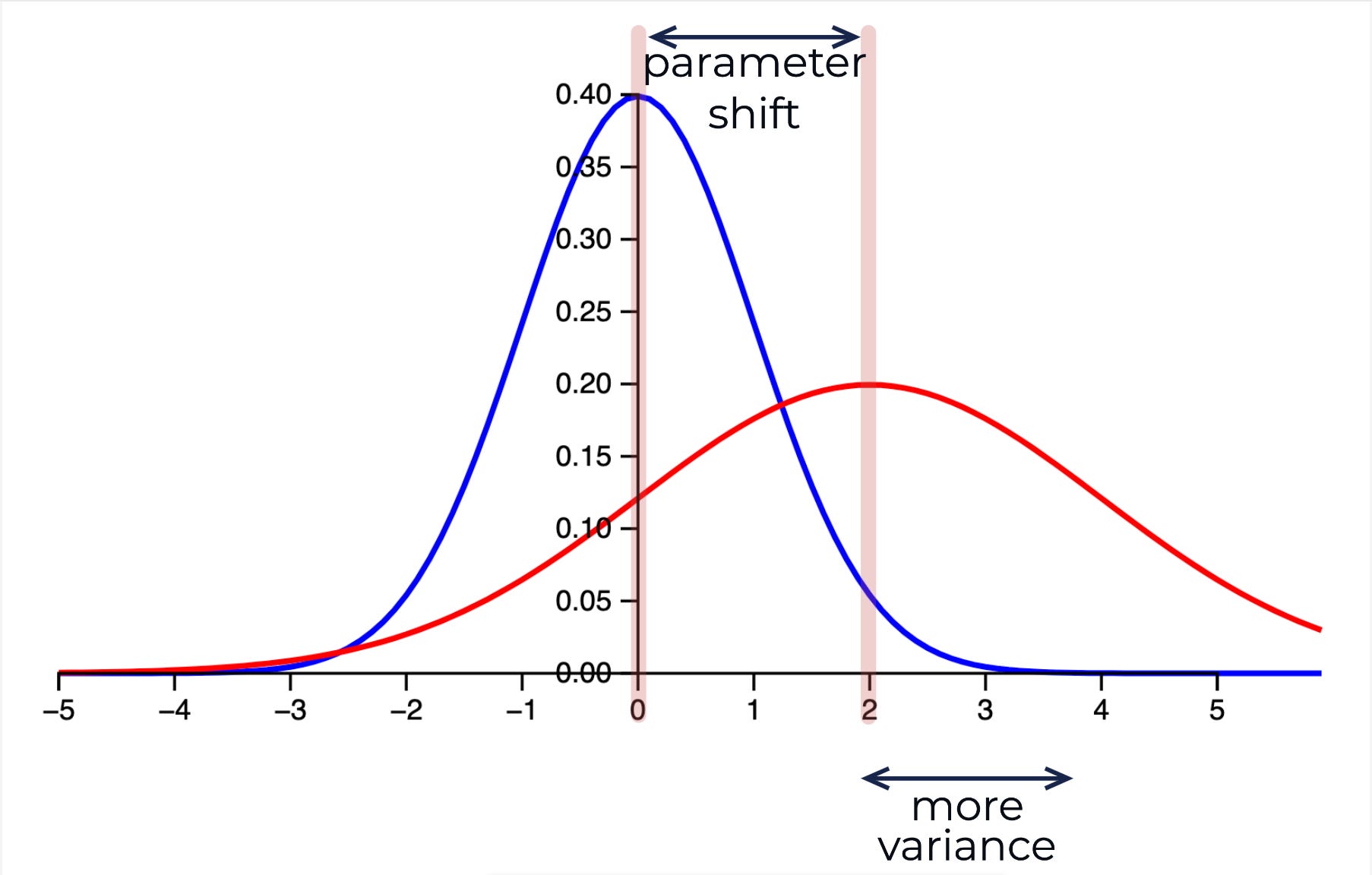
Given two Gaussian distributions that represent the probability distributions for some outcome, we can measure the amount of entropy or ‘surprise’ between the distributions. This comes from information theory and is the basis for the KL divergence, a distance between distributions used as part of the Variational inference approach described below.
This is a launching point and very basic introduction to one of the many ways we can detect statistical shifts in time series data; change points in non-stationary data and how this may be relevant to dynamical systems with irreversible dynamics and critical transitions.
(Mean + Variance Shift)
Discovering Latent States
In this post I will describe a method that uses Scikit-learn to reveal latent states in time series data using a stochastic Dirichlet process mixture model. This is an implementation of Variational inference, an optimization approach inspired by statistical physics.
Variational methods have a long tradition in statistical physics. The mean field method was originally applied to model spin glasses, which are certain types of disordered magnets where the magnetic spins of the atoms are not aligned in a regular pattern. A simple example for such a spin glass model is the Ising model, a model of binary variables on a lattice with pairwise couplings. To estimate the resulting statistical distribution of spin states, a simpler, factorized distribution is used as a proxy. This is done with the goal of approximating the marginal probabilities of the spins pointing up or down (also called ’magnetization’) as well as possible, while ignoring all correlations between the spins. The many interactions of a given spin with its neighbors are replaced by a single interaction between a spin and the effective magnetic field (a.k.a. mean field) of all other spins. This explains the name origin. Physicists typically denote the negative log posterior as an energy or Hamiltonian function. This language has been adopted by the machine learning community for approximate inference in both directed and undirected models.
Advances in Variational Inference (IEEE)
It is a generative model that first clusters the data by mean and covariance, and then can generate samples from the posterior distribution. The problem of finding the posterior is an instance of a more general problem that Variational inference solves for efficiently, and what it provides is only an approximation to the posterior. It allows one to construct a data generating process of the learned phenomenon.
(Posterior Distribution)
We are essentially answering the question: what hidden partitions would have made the observed data most probable to observe? It is achieved by optimizing the likelihood of the data x given the parameters that we assume for each partition.
(Hidden Partitions)
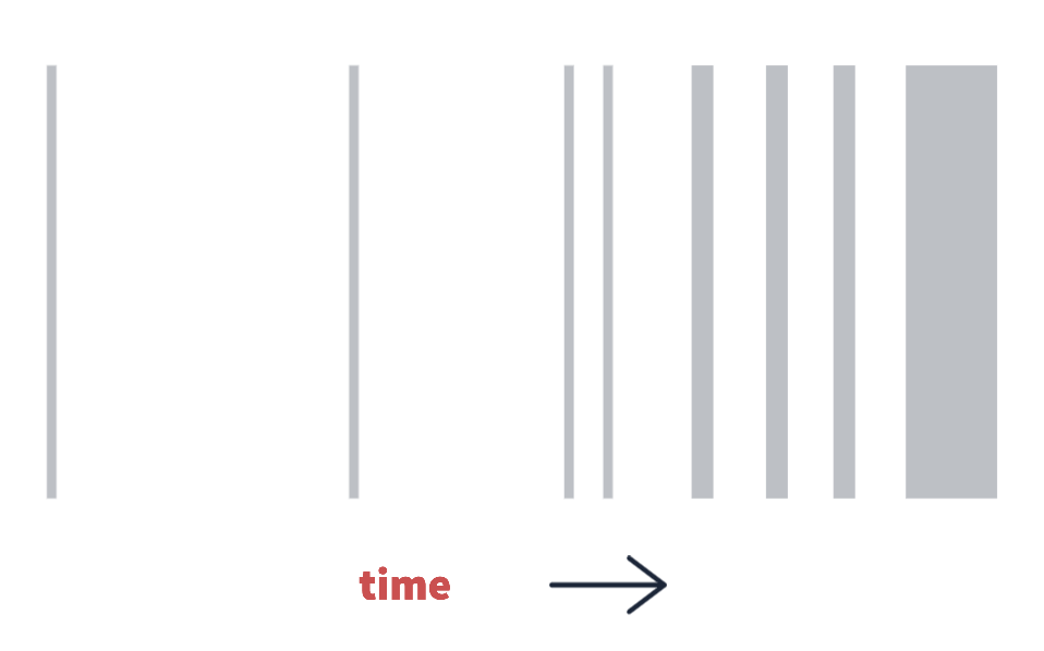
(above: a latent state time partition, growing in frequency and duration sequentially with time)
Time Series Latent States
In this scenario a time series will be a time-ordered sequence of random values that follow some distribution with mean mu and variance sigma squared,
(Normal Distribution - Prior)
Considering a portfolio optimization task of designing exposures to random time-ordered asset returns, we end up tracking three data streams over time, envisioned as a 3d environment for simplicity.
(Asset Data)
We could examine if mean and covariance relationships exist between these asset classes such that their returns offset each other at least some of the time, or they may be correlated. We can investigate the time-varying nature of the correlations and covariance matrix. If one asset’s mean is causing it to trend in the opposite direction of another, this is also relevant.
(List of Means)
(Covariance Matrix)
We are simply finding if time points occurring far apart or adjacent in time are related by similar statistical parameters. A pattern that occurs, disappears, and re-occurs. Adjacent and non-adjacent time points may belong to the same partition because of their related statistical parameters, they are hence part of the same latent state.
We use the model to find the parameters that produce a distribution over the latent states, a distribution over distributions. This is the exact same thing as a distribution of clusters, clusters are states and states are clusters.
Dirichlet Process Gaussian Mixture
How shall we choose the number of clusters? The Dirichlet process is a non-parametric approach where the number of clusters need not be known in advance, because the most likely number of clusters will be learnt from the data as well. Even though a Gaussian may not be a perfect representation of the kurtosis and long-tailed nature of the data, we can learn as many clusters as are necessary to characterize important differences between statistical regimes in the data, subject to some model tweaking.
Now we will tackle how Variational inference frames all of this as an optimization problem. This is the posterior distribution function for the probability of parameters theta (𝜽) given the observed data x with cluster families i=1 through to the length n. The likelihood of the parameters at value x is given by a sum over gaussian functions with parameters mean mu, covariance matrix Sigma, and a weight ω. The summation symbol shows that the likelihood for the observed data x is computed from a mixture of weighted normal distributions.
(Mixture Model)
The gaussian distribution function with mean mu and covariance matrix Sigma being represented by this term with an additional weight term (ω). These are all the parameters that the model updates during optimization: the weights, the mixture means, and the mixture covariance matrices.
(Model Parameters)
This weight term (ω) is important. It means that once we truncate any clusters with negligible weights, the cluster assignments at each time point become represented by a finite length vector of weights summing to 1, such that we are probabilistically in each cluster.
(Probabilistic Cluster Assignment)
We can consider the discrete state assignment to simply be the highest probability weight at that time point which is the argmax of the probabilistic weights.
Mean-Field Variational Inference
To keep it simple let’s assume that every time point has an equal likelihood of belonging to any state. The parameters of the model can then be updated using a process similar to Expectation-Maximization until the ELBO (Evidence Lower Bound) has been maximized, which is equivalent to minimizing the Kullback–Leibler divergence.
(KL Divergence)
The entropy or amount of ‘surprise’ between our target (the true posterior) and the variational latent parameters q is minimized, which is the same as saying we have maximized log likelihood of those parameters given the data, which is what the algorithm actually does. Maximizing log likelihood using Jensen’s inequality,
(Jensen’s Inequality)
is equivalent to minimizing the KL divergence as shown in equation (11),
(KL Divergence)
The reality is that we cannot compute the posterior exactly, as it is an intractable problem. So the variational distribution q is used as an approximation to understand the true posterior. I recommend this lecture and this paper for in depth step-by-step walkthroughs of deriving this algorithm.
Generating Data
In the linked image and notebook below, the shaded regions on the chart show the most frequently occurring latent state. The model re-creates the prevailing theme of 2022 in a synthetic way: commodities rising while tech and treasuries tend to fall. The effect was more significant in the first half of the year, versus the last, where then the offsetting regime became more frequent. There is interpretable economic significance to this discovery from a purely descriptive point of view.
(Experiment 1)
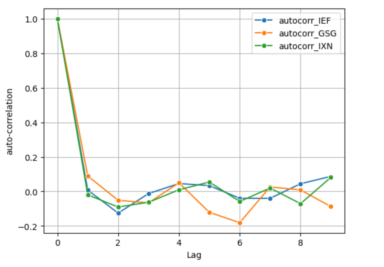
1st-order differenced log returns, the standard way of producing log returns which can make the series mean stationary but removes memory e.g. auto-correlation. This only removes one unit root. At a lag value of just 1, the series’ auto-correlations are nearly 0 or below 0 and at further lags there is some auto-correlation but it is low.
(Log Returns)
(ACF Function)
The generative sample re-creates the prevailing theme of 2022 in a synthetic way with Markov sampling — each state is sampled without any dependence on the state that came before it, but all states have an overall probability and frequency of occurrence that reflects their posterior weight. States are shown below overlaid on the cumulative sum of the log returns, converted back to log price after sampling.
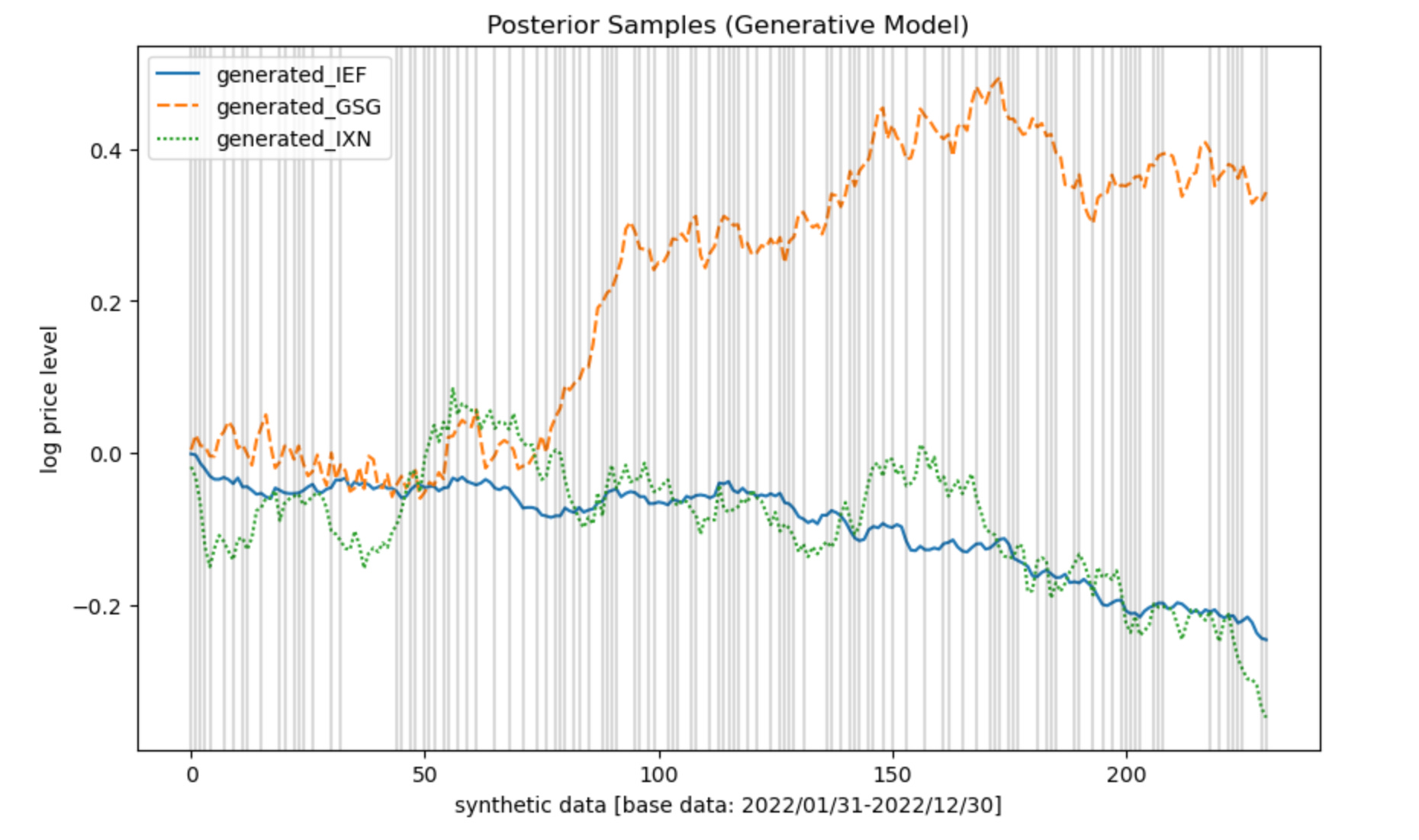
Notebook: Variational Inference - Sampling the Generative Model
(Experiment 2)
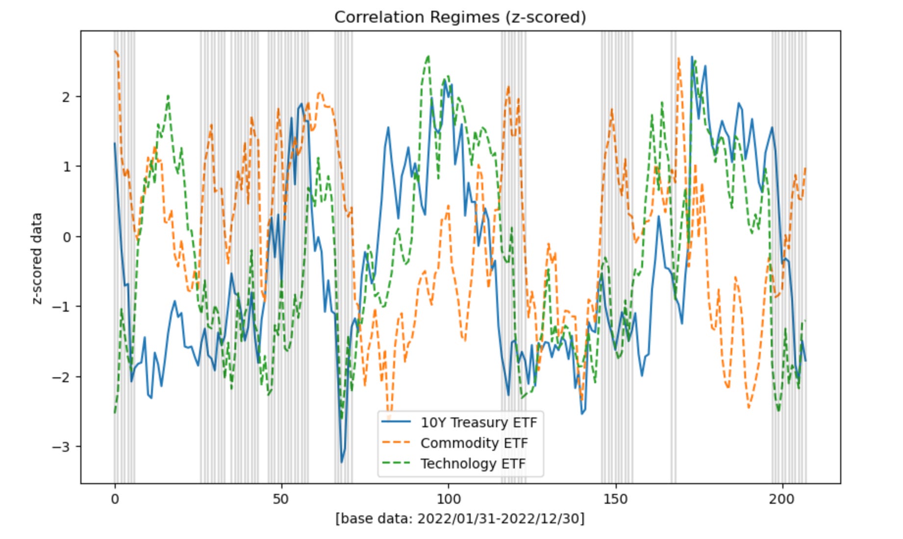
In this next experiment log prices are Z-scored based on a rolling window where the Z-score calculation considers the data within the look back window only. This produces auto-correlation because with a rolling parameter present values are directly influenced by further back, historical values, by the very construction of the rolling window. A cyclical pattern of mean reversion also emerges, since periods with large moves cannot last forever, especially when measured against the standard deviation and mean of the recent past.
Given current value at time x_t and window look back length w, parameters mu and sigma for the Z-score calculation are limited to the window t - w through t,
(Z-Score)
The model finds clusters with parameters of the same root economic significance discussed earlier: periods where commodities tend to do well are offset by tech/treasuries doing poorly and vice versa.
Notebook: Variational Inference - Discovering Latent States
Auto-correlation & Markovian Dynamics
There is a caveat to this approach. The generative model does not handle auto-correlated processes in a way that takes into account the rate of auto-correlation decay after a sample. In cases where we cannot assume independence or uniformity across time, the generative model won’t recreate any short or long memory effects present in the data generating process. It cannot recreate the long-range dependence that we intentionally introduced in Experiment 2.
Each new state in the data generating process is sampled without any dependence on the state that came before it. This is why typically when working with the data in machine learning tasks we try to make it stationary and IID first, such as with a differencing process that also removes memory, although imperfectly, as we did in Experiment 1. In future posts I will dive into Hidden Markov Models and other state-space models that address this dependency.
Back to Economic Significance
This model recreates an interpretable economic theme we can now see clearly in the distributional properties of the data. If we are dealing with the higher level distribution over distributions, then what we truly care about is what state we are observing in the here and now, what is the significance of that, and what might be the probability over time of diffusion or of switching to another state.
Commodities rising while tech and treasuries tend to fall is characteristic of an economic system going through major shifts that we know: a shift from loose to restrictive monetary policy and quantitative tightening, rising interest rates, a commodity and energy shock brought on by the pandemic supply restrictions and Ukraine war, and historic levels of inflation.
References & Further Reading
Variational Inference
David M. Blei
Advances in Variational Inference
IEEE
Variational Inference for Dirichlet process mixtures
David M. Blei, Michael I. Jordan
Dirichlet Process
Yee Whye Teh, University College London
EM Algorithm
Tengyu Ma and Andrew Ng
Long Memory and Regime Switching
Francis X. Diebold, Atsushi Inoue
Macroeconomic Regimes and Regime Shifts
James D. Hamilton
The Dripping Faucet as a Model Chaotic System
Robert Shaw
Regimes in Simple Systems
Edward Norton Lorenz
& more in the README: https://github.com/regimelab/notebooks/?tab=readme-ov-file#further-reading--inspiration