

Stagflation is an economic condition where inflation remains stubbornly elevated while the job market deteriorates, or there are other coinciding signs of inflation and disinflation/deflation simultaneously. Unemployment may rise in a time when the Fed is constrained by inflation being too high to lower rates or ease monetary policy. In an era of fiscal dominance that might just be the problem.
The Shape of Stagflation
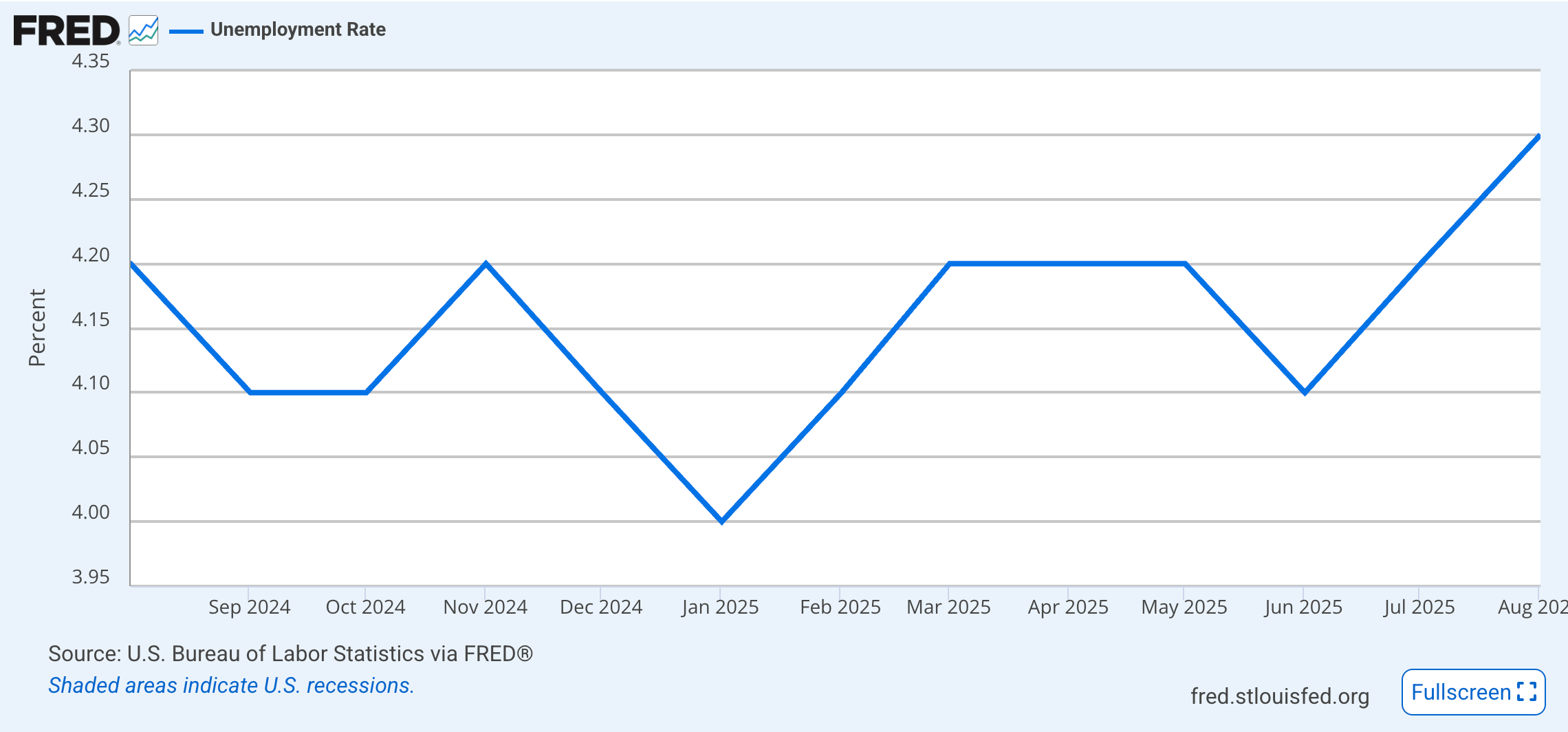
In this post I will be using Principal Component Analysis (PCA) to generate principal eigenportfolios that may show stagflation dynamics in recent market action. There have been a series of strong inflationary numbers coming out at the same time that unemployment may be rising, a condition consistent with stagflation. Unemployment has finally broken above the 4.2% ceiling it had been hitting for some time.
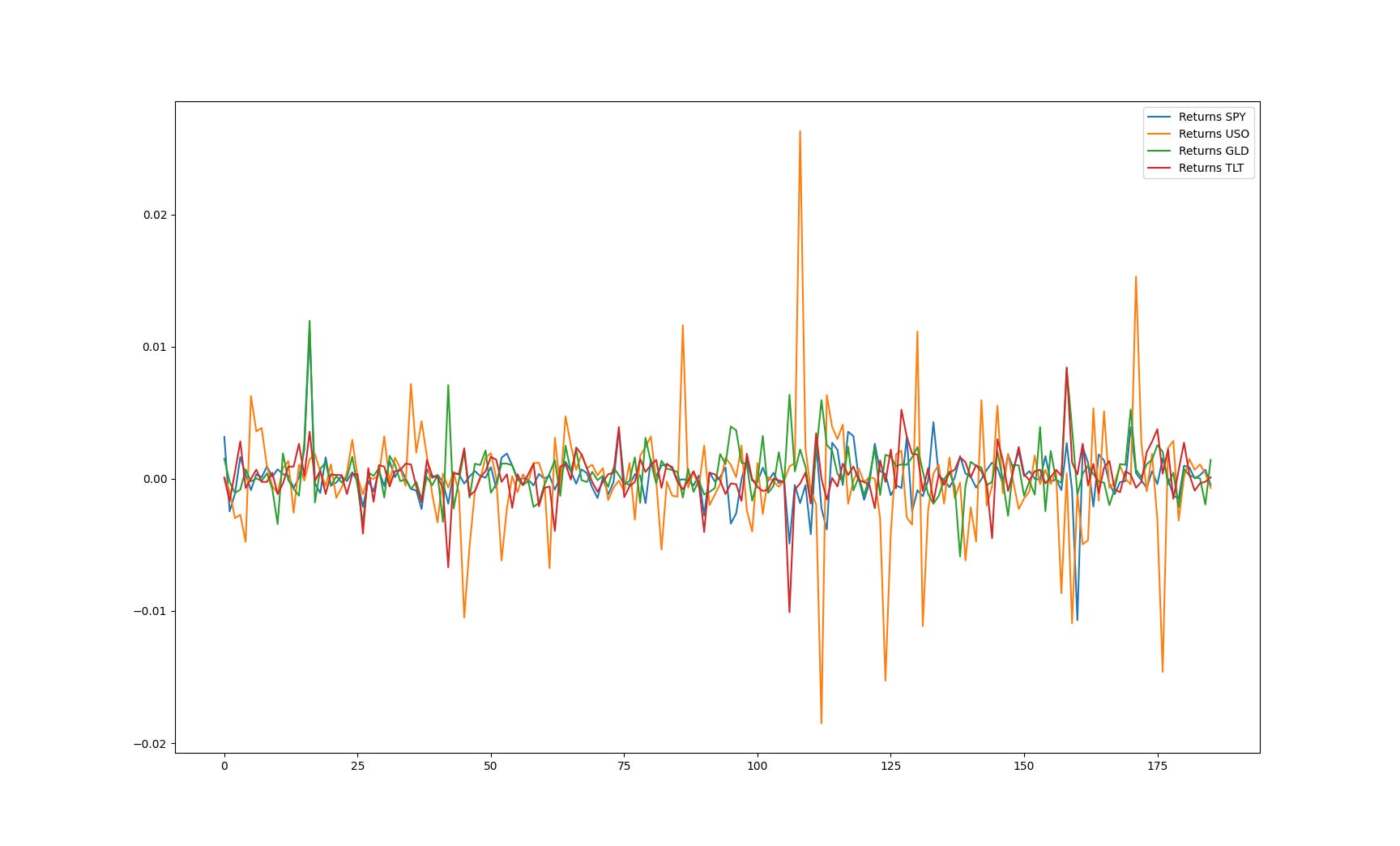
The task is to see if we can capture the shape of this data using machine learning. Let’s dive a bit deeper into the market dynamics behind stagflation by analyzing a simple set of assets, the following ETF tickers which represent major asset classes: Equities, Oil, Gold, and long term Treasuries.
[“SPY", "USO", "GLD", "TLT"] In a stagflation scenario we will see Gold outperform and Treasuries as well as Equities probably struggle since yields will see upward pressure from investors demanding higher inflation risk premium. This is at the same time as they seek Gold to hedge against the Fed losing control of the situation entirely.
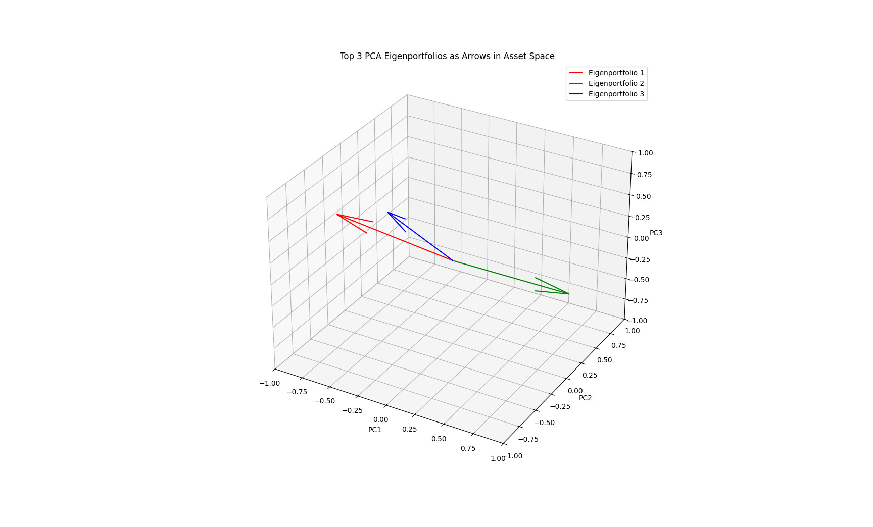
Let’s start by taking a look at the top 3 PCA eigenvectors, which will be treated as weight vectors which form a portfolio of these assets. The weights will be normalized to represent a long-only portfolio.
returns = np.diff(np.log(closes))The covariance matrix of the log returns is used to fit the model. The eigenports function defines an implementation of PCA fit on the covariance matrix of the log returns.
def eigenports(rets, num_components=3):
  ‘’‘
  reduce dimensionality via PCA
  generate orthonormal investment Universes (principal Eigenportfolios)

  rets - returns matrix
  num_components - how many PCA vectors to discover
  ‘’‘
  eigenvecs = []
  cols = rets.columns.unique()
  feat_num = len(cols)

  pca = PCA(n_components=num_components)
  components = pca.fit_transform(rets[cols].cov())

  for M in range(num_components):
    eigenvec = pd.Series(index=range(feat_num), data=pca.components_[M])
    eigenvecs.append(eigenvec)

  return eigenvecs, pca, components

# Fetch returns for all tickers and align lengths
all_returns = [fetch_hourly_returns(tkr) for tkr in TICKERS]
min_len = min(len(r) for r in all_returns)
all_returns = [r[-min_len:] for r in all_returns]

...

# Get eigenportfolios
returns_matrix = pd.DataFrame(all_returns).transpose()
eigenvectors, pca, components = eigenports(returns_matrix)

# Normalize eigenportfolios to long only portfolios:
# Take absolute values and normalize to sum to one per eigenvector
eigenvectors_long_only = np.abs(eigenvectors)
eigenvectors_long_only /= eigenvectors_long_only.sum(axis=1, keepdims=True)
Visualize the log returns of each asset.
Visualize the eigenvectors in a 3d space. One particular eigenvector, Eigenportfolio 2, stands out as directionally orthogonal to the other two. This is a simplified, toy example, but these orthogonal vectors can be treated as orthonormal investment universes as written by Marcos Lopez de Prado and Marco Avallaneda et al in the literature cited below.
Lastly the performance of these weight vectors treated as portfolios you would actually hold is plotted for the past 18 trading days using the cumulative sum of the sorted return.
Sorted Returns
I will look at the comparative performance of the eigenportfolios in terms of the sorted log returns instead of the time-ordered returns. This is a variation on the traditional approach, but I believe it still works because we are more interested in the distributional shape of the data as opposed to exactly where all the volatility is in sequential time. It becomes much like a CDF but ultimately measures performance not probability.
Volatility and non-stationarity in sequential time introduce sensitivity to initial conditions when evaluating portfolio growth. Since there is path dependence a portfolio that gets off to a bad start will have a hard time catching up with the others over some arbitrary time period, yet it’s distributional properties may outperform those others over a longer, more important time frame.
Using sorted returns removes the possibility of compounding from the analysis. There is no concept of compounding portfolio growth over time instead just additive performance for the purpose of distributional analysis within a window, which is intentional.
Visualizing the data this way also emphasizes the tails of the distribution.
Top 3 Eigenportfolio Weights (Long-Only Normalized):
Eigenportfolio 1: [0.079 0.757 0.092 0.072]
Eigenportfolio 2: [0.157 0.015 0.507 0.322]
Eigenportfolio 3: [0.548 0.013 0.067 0.372]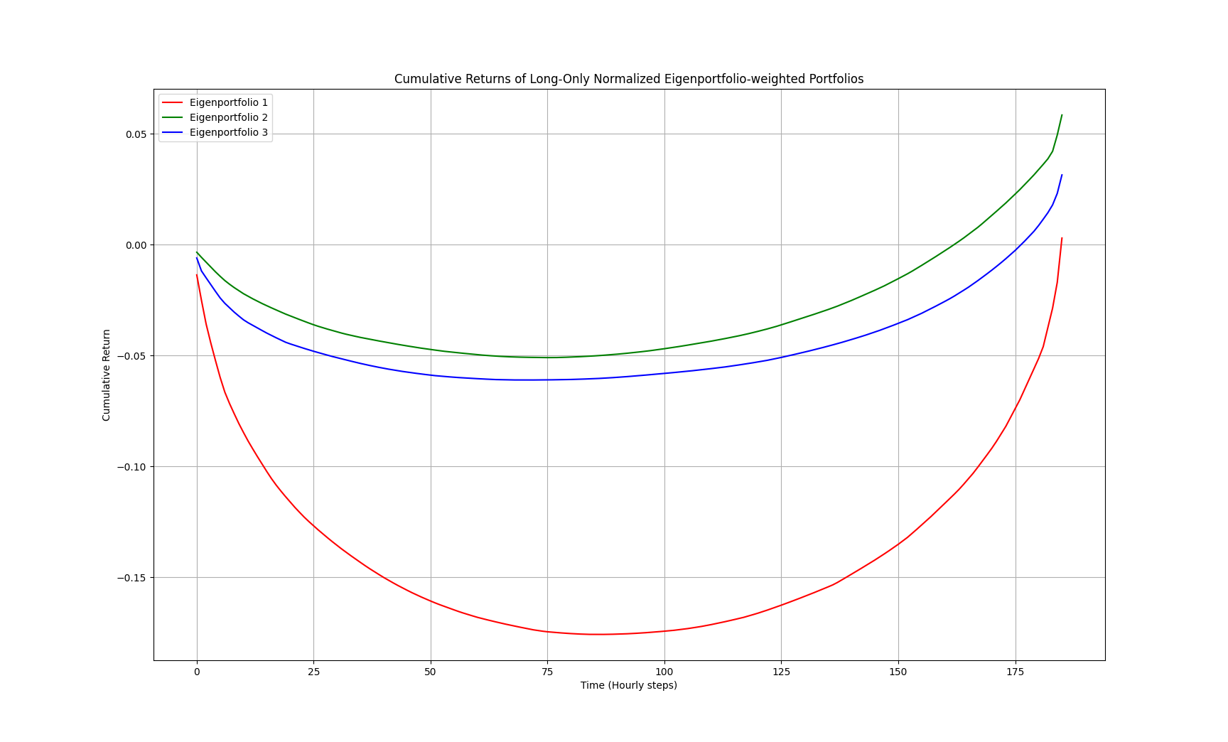
We can see in the chart above that portfolio performances vary in their volatility since the depth of the ‘smile’ represents how volatile that series is. The top eigenportfolio is the most volatile, and the portfolios become less volatile as you move deeper into the orthogonal set of eigenvectors. They are essentially ranked by their volatility because the top eigenvector explains the most variance, and so on.
It’s also important to note that a less volatile portfolio can end up beating a more volatile one, which would offer and even better Sharpe or Sortino ratio, a much better risk-to-return.
Source code:
https://github.com/regimelab/the-shape-of-stagflation/
2nd Principal Component
The 2nd principal component breaks out and outperforms the others but the 3rd component is a close second. The 1st principal component does particularly poorly being heavily weighted in USO. In a classical inflation scenario with growth we should see oil outperform, that this doesn’t show up signals an additional possible trait of stagflation. A portfolio heavy in SPY and TLT is the close second.
Often the market prices in certain macroeconomic expectations in advance, and those do end up eventually manifesting after a lag. If CPI comes in hot later this week that will further solidify the case for stagflation.
References & Further Reading
PCA Scikit-Learn
Unemployment Rate Federal Reserve
Managing Risks in a Risk-On/Risk-Off Environment Marcos Lopez de Prado
Principal Eigenportfolios for U.S. Equities Marco Avallaneda, Brian Healy, Andrew Papanicolaou, George Papanicoalou